Policy

Policy#

In reinforcement learning, the agent interacts with environments to improve itself. In this tutorial we will concentrate on the agent part. In Tianshou, both the agent and the core DRL algorithm are implemented in the Policy module. Tianshou provides more than 20 Policy modules, each representing one DRL algorithm. See supported algorithms here.

The agents interacting with the environment

All Policy modules inherit from a BasePolicy Class and share the same interface.

Creating your own Policy#

We will use the simple PGPolicy, also called REINFORCE algorithm Policy, to show the implementation of a Policy Module. The Policy we implement here will be a scaled-down version of PGPolicy in Tianshou.

Protocols#

Note: as we learned in tutorial L1_batch, Tianshou uses Batch to store data. Batch is a dataclass that can store any data you want. In order to have more control about what kind of batch data is expected and produced in each processing step we use protocols.
For example, BatchWithReturnsProtocol specifies that the batch should have fields obs, act, rew, done, obs_next, info and returns. This is not only for type checking, but also for IDE support. To learn more about protocols, please refer to the official documentation (PEP 544) or to mypy documentation (Protocols).

Initialization#

Firstly we create the PGPolicy by inheriting from BasePolicy in Tianshou.

class PGPolicy(BasePolicy):
    """Implementation of REINFORCE algorithm."""

    def __init__(self) -> None:
        super().__init__(
            action_space=action_space,
            observation_space=observation_space,
        )

The Policy Module mainly does two things:

policy.forward() receives observation and other information (stored in a Batch) from the environment and returns a new Batch containing the next action and other information.
policy.update() receives training data sampled from the replay buffer and updates the policy network. It returns a dataclass containing logging details.

policy.forward() and policy.update()

We also need to take care of the following things:

Since Tianshou is a Deep RL libraries, there should be a policy network and a Torch optimizer in our Policy Module.
In Tianshou’s BasePolicy, Policy.update() first calls Policy.process_fn() to preprocess training data and computes quantities like episodic returns (gradient free), then it will call Policy.learn() to perform the back-propagation.
Each Policy is accompanied by a dedicated implementation of TrainingStats , which store details of each training step.

This is how we get the implementation below.

class PGPolicy(BasePolicy[TPGTrainingStats]):
    """Implementation of REINFORCE algorithm."""

    def __init__(
        self, 
        actor: torch.nn.Module, 
        optim: torch.optim.Optimizer, 
        action_space: gym.Space
    ):
        super().__init__(
            action_space=action_space,
            observation_space=observation_space
        )
        self.actor = model
        self.optim = optim

    def process_fn(
        self, 
        batch: RolloutBatchProtocol, 
        buffer: ReplayBuffer, 
        indices: np.ndarray
    ) -> BatchWithReturnsProtocol:
        """Compute the discounted returns for each transition."""
        return batch

    def forward(
        self, 
        batch: ObsBatchProtocol,
        state: dict | BatchProtocol | np.ndarray | None = None,
        **kwargs: Any
    ) -> DistBatchProtocol:
        """Compute action over the given batch data."""
        act = None
        return Batch(act=act)

    def learn(
        self,
        batch: BatchWithReturnsProtocol, 
        batch_size: int | None, 
        repeat: int,
        *args: Any,
        **kwargs: Any,
    ) -> TPGTrainingStats:
        """Perform the back-propagation."""
        return PGTrainingStats(loss=loss_summary_stat)

Policy.forward()#

According to the equation of REINFORCE algorithm in Spinning Up’s documentation, we need to map the observation to an action distribution in action space using the neural network (self.actor).

Let us suppose the action space is discrete, and the distribution is a simple categorical distribution.

def forward(
    self,
    batch: ObsBatchProtocol,
    state: dict | BatchProtocol | np.ndarray | None = None,
    **kwargs: Any,
) -> DistBatchProtocol:
    """Compute action over the given batch data."""
    logits, hidden = self.actor(batch.obs, state=state)
    dist = self.dist_fn(logits)
    act = dist.sample()
    result = Batch(logits=logits, act=act, state=hidden, dist=dist)
    return result

Policy.process_fn()#

Now that we have defined our actor, if given training data we can set up a loss function and optimize our neural network. However, before that, we must first calculate episodic returns for every step in our training data to construct the REINFORCE loss function.

Calculating episodic return is not hard, given ReplayBuffer.next() allows us to access every reward to go in an episode. A more convenient way would be to simply use the built-in method BasePolicy.compute_episodic_return() inherited from BasePolicy.

def process_fn(
    self,
    batch: RolloutBatchProtocol,
    buffer: ReplayBuffer,
    indices: np.ndarray,
) -> BatchWithReturnsProtocol:
    """Compute the discounted returns for each transition."""
    v_s_ = np.full(indices.shape, self.ret_rms.mean)
    returns, _ = self.compute_episodic_return(batch, buffer, indices, v_s_=v_s_, gamma=0.99, gae_lambda=1.0)
    batch.returns = returns
    return batch

BasePolicy.compute_episodic_return() could also be used to compute GAE. Another similar method is BasePolicy.compute_nstep_return(). Check the source code for more details.

Policy.learn()#

Data batch returned by Policy.process_fn() will flow into Policy.learn(). Finally, we can construct our loss function and perform the back-propagation. The method should look something like this:

def learn(
    self,
    batch: BatchWithReturnsProtocol,
    batch_size: int | None,
    repeat: int,
    *args: Any,
    **kwargs: Any,
) -> TPGTrainingStats:
    """Perform the back-propagation."""
    losses = []
    split_batch_size = batch_size or -1
    for _ in range(repeat):
        for minibatch in batch.split(split_batch_size, merge_last=True):
            self.optim.zero_grad()
            result = self(minibatch)
            dist = result.dist
            act = to_torch_as(minibatch.act, result.act)
            ret = to_torch(minibatch.returns, torch.float, result.act.device)
            log_prob = dist.log_prob(act).reshape(len(ret), -1).transpose(0, 1)
            loss = -(log_prob * ret).mean()
            loss.backward()
            self.optim.step()
            losses.append(loss.item())
    loss_summary_stat = SequenceSummaryStats.from_sequence(losses)

    return PGTrainingStats(loss=loss_summary_stat)

Implementation#

Now we can assemble the methods and form a PGPolicy. The outputs of learn will be collected to a dedicated dataclass.

class PGPolicy(BasePolicy[TPGTrainingStats]):
    """Implementation of REINFORCE algorithm."""

    def __init__(
        self,
        *,
        actor: torch.nn.Module,
        optim: torch.optim.Optimizer,
        dist_fn: TDistributionFunction,
        action_space: gym.Space,
        discount_factor: float = 0.99,
        observation_space: gym.Space | None = None,
    ) -> None:
        super().__init__(
            action_space=action_space,
            observation_space=observation_space,
        )
        self.actor = actor
        self.optim = optim
        self.dist_fn = dist_fn
        assert 0.0 <= discount_factor <= 1.0, "discount factor should be in [0, 1]"
        self.gamma = discount_factor
        self.ret_rms = RunningMeanStd()

    def process_fn(
        self,
        batch: RolloutBatchProtocol,
        buffer: ReplayBuffer,
        indices: np.ndarray,
    ) -> BatchWithReturnsProtocol:
        """Compute the discounted returns (Monte Carlo estimates) for each transition.

        They are added to the batch under the field `returns`.
        Note: this function will modify the input batch!
        """
        v_s_ = np.full(indices.shape, self.ret_rms.mean)
        # use a function inherited from BasePolicy to compute returns
        # gae_lambda = 1.0 means we use Monte Carlo estimate
        batch.returns, _ = self.compute_episodic_return(
            batch,
            buffer,
            indices,
            v_s_=v_s_,
            gamma=self.gamma,
            gae_lambda=1.0,
        )
        batch: BatchWithReturnsProtocol
        return batch

    def forward(
        self,
        batch: ObsBatchProtocol,
        state: dict | BatchProtocol | np.ndarray | None = None,
        **kwargs: Any,
    ) -> DistBatchProtocol:
        """Compute action over the given batch data by applying the actor.

        Will sample from the dist_fn, if appropriate.
        Returns a new object representing the processed batch data
        (contrary to other methods that modify the input batch inplace).
        """
        logits, hidden = self.actor(batch.obs, state=state)

        if isinstance(logits, tuple):
            dist = self.dist_fn(*logits)
        else:
            dist = self.dist_fn(logits)

        act = dist.sample()
        return cast(DistBatchProtocol, Batch(logits=logits, act=act, state=hidden, dist=dist))

    def learn(  # type: ignore
        self,
        batch: BatchWithReturnsProtocol,
        batch_size: int | None,
        repeat: int,
        *args: Any,
        **kwargs: Any,
    ) -> TPGTrainingStats:
        losses = []
        split_batch_size = batch_size or -1
        for _ in range(repeat):
            for minibatch in batch.split(split_batch_size, merge_last=True):
                self.optim.zero_grad()
                result = self(minibatch)
                dist = result.dist
                act = to_torch_as(minibatch.act, result.act)
                ret = to_torch(minibatch.returns, torch.float, result.act.device)
                log_prob = dist.log_prob(act).reshape(len(ret), -1).transpose(0, 1)
                loss = -(log_prob * ret).mean()
                loss.backward()
                self.optim.step()
                losses.append(loss.item())

        loss_summary_stat = SequenceSummaryStats.from_sequence(losses)

        return PGTrainingStats(loss=loss_summary_stat)  # type: ignore[return-value]

Use the policy#

Note that BasePolicy itself inherits from torch.nn.Module. As a result, you can consider all Policy modules as a Torch Module. They share similar APIs.

Firstly we will initialize a new PGPolicy.

state_shape = 4
action_shape = 2
# Usually taken from an env by using env.action_space
action_space = gym.spaces.Box(low=-1, high=1, shape=(2,))
net = Net(state_shape, hidden_sizes=[16, 16], device="cpu")
actor = Actor(net, action_shape, device="cpu").to("cpu")
optim = torch.optim.Adam(actor.parameters(), lr=0.0003)
dist_fn = torch.distributions.Categorical

policy: BasePolicy
policy = PGPolicy(actor=actor, optim=optim, dist_fn=dist_fn, action_space=action_space)

PGPolicy shares same APIs with the Torch Module.

print(policy)
print("========================================")
for param in policy.parameters():
    print(param.shape)

PGPolicy(
  (actor): Actor(
    (preprocess): Net(
      (model): MLP(
        (model): Sequential(
          (0): Linear(in_features=4, out_features=16, bias=True)
          (1): ReLU()
          (2): Linear(in_features=16, out_features=16, bias=True)
          (3): ReLU()
        )
      )
    )
    (last): MLP(
      (model): Sequential(
        (0): Linear(in_features=16, out_features=2, bias=True)
      )
    )
  )
)
========================================
torch.Size([16, 4])
torch.Size([16])
torch.Size([16, 16])
torch.Size([16])
torch.Size([2, 16])
torch.Size([2])

Making decision#

Given a batch of observations, the policy can return a batch of actions and other data.

obs_batch = Batch(obs=np.ones(shape=(256, 4)))
dist_batch = policy(obs_batch)  # forward() method is called
print("Next action for each observation: \n", dist_batch.act)
print("Dsitribution: \n", dist_batch.dist)

Next action for each observation: 
 tensor([0, 1, 0, 1, 1, 1, 1, 1, 0, 1, 1, 1, 1, 0, 1, 0, 0, 0, 0, 1, 0, 1, 0, 1,
        0, 1, 0, 1, 1, 1, 0, 0, 1, 0, 0, 0, 1, 1, 0, 0, 0, 1, 0, 1, 0, 0, 1, 1,
        0, 1, 1, 0, 1, 0, 1, 0, 1, 0, 0, 0, 0, 1, 1, 0, 1, 0, 1, 0, 1, 1, 0, 0,
        1, 0, 1, 0, 1, 1, 0, 0, 0, 0, 1, 0, 1, 0, 0, 1, 0, 0, 1, 1, 1, 0, 0, 1,
        1, 1, 0, 1, 1, 1, 1, 1, 0, 0, 0, 1, 1, 1, 1, 1, 0, 1, 0, 1, 1, 1, 1, 0,
        1, 1, 1, 1, 1, 0, 1, 0, 0, 0, 0, 0, 0, 1, 1, 0, 1, 0, 0, 1, 0, 1, 1, 0,
        0, 1, 1, 0, 1, 1, 0, 0, 1, 1, 0, 0, 0, 0, 1, 1, 1, 1, 1, 0, 1, 0, 0, 1,
        1, 1, 0, 0, 0, 0, 1, 0, 1, 1, 0, 0, 0, 1, 0, 0, 0, 1, 0, 1, 0, 0, 1, 1,
        1, 0, 0, 0, 0, 0, 1, 1, 1, 1, 1, 1, 0, 1, 1, 0, 0, 1, 1, 1, 1, 0, 1, 0,
        1, 0, 1, 0, 0, 1, 1, 0, 1, 0, 1, 0, 0, 0, 1, 1, 1, 1, 0, 0, 1, 1, 1, 1,
        0, 1, 0, 0, 0, 1, 0, 0, 1, 0, 1, 0, 0, 1, 0, 1])
Dsitribution: 
 Categorical(probs: torch.Size([256, 2]))

Save and Load models#

Naturally, Tianshou Policy can be saved and loaded like a normal Torch Network.

torch.save(policy.state_dict(), "policy.pth")
assert policy.load_state_dict(torch.load("policy.pth"))

Algorithm Updating#

We have to collect some data and save them in the ReplayBuffer before updating our agent(policy). Typically we use collector to collect data, but we leave this part till later when we have learned the Collector in Tianshou. For now we generate some fake data.

Generating fake data#

Firstly, we need to “pretend” that we are using the “Policy” to collect data. We plan to collect 10 data so that we can update our algorithm.

dummy_buffer = ReplayBuffer(size=10)
print(dummy_buffer)
print(f"maxsize: {dummy_buffer.maxsize}, data length: {len(dummy_buffer)}")
env = gym.make("CartPole-v1")

ReplayBuffer()
maxsize: 10, data length: 0

Now we are pretending to collect the first episode. The first episode ends at step 3 (perhaps because we are performing too badly).

obs, info = env.reset()
for i in range(3):
    act = policy(Batch(obs=obs[np.newaxis, :])).act.item()
    obs_next, rew, _, truncated, info = env.step(act)
    # pretend ending at step 3
    terminated = i == 2
    info["id"] = i
    dummy_buffer.add(
        Batch(
            obs=obs,
            act=act,
            rew=rew,
            terminated=terminated,
            truncated=truncated,
            obs_next=obs_next,
            info=info,
        ),
    )
    obs = obs_next

print(dummy_buffer)

ReplayBuffer(
    obs: array([[ 0.02516632, -0.03213277,  0.00827677,  0.00761275],
                [ 0.02452366, -0.22737244,  0.00842903,  0.30289558],
                [ 0.01997622, -0.03237162,  0.01448694,  0.01288284],
                [ 0.        ,  0.        ,  0.        ,  0.        ],
                [ 0.        ,  0.        ,  0.        ,  0.        ],
                [ 0.        ,  0.        ,  0.        ,  0.        ],
                [ 0.        ,  0.        ,  0.        ,  0.        ],
                [ 0.        ,  0.        ,  0.        ,  0.        ],
                [ 0.        ,  0.        ,  0.        ,  0.        ],
                [ 0.        ,  0.        ,  0.        ,  0.        ]],
               dtype=float32),
    act: array([0, 1, 0, 0, 0, 0, 0, 0, 0, 0]),
    rew: array([1., 1., 1., 0., 0., 0., 0., 0., 0., 0.]),
    terminated: array([False, False,  True, False, False, False, False, False, False,
                       False]),
    truncated: array([False, False, False, False, False, False, False, False, False,
                      False]),
    obs_next: array([[ 0.02452366, -0.22737244,  0.00842903,  0.30289558],
                     [ 0.01997622, -0.03237162,  0.01448694,  0.01288284],
                     [ 0.01932878, -0.22769831,  0.0147446 ,  0.31010112],
                     [ 0.        ,  0.        ,  0.        ,  0.        ],
                     [ 0.        ,  0.        ,  0.        ,  0.        ],
                     [ 0.        ,  0.        ,  0.        ,  0.        ],
                     [ 0.        ,  0.        ,  0.        ,  0.        ],
                     [ 0.        ,  0.        ,  0.        ,  0.        ],
                     [ 0.        ,  0.        ,  0.        ,  0.        ],
                     [ 0.        ,  0.        ,  0.        ,  0.        ]],
                    dtype=float32),
    info: Batch(
              id: array([0, 1, 2, 0, 0, 0, 0, 0, 0, 0]),
          ),
    done: array([False, False,  True, False, False, False, False, False, False,
                 False]),
)

Now we are pretending to collect the second episode. At step 7 the second episode still doesn’t end, but we are unwilling to wait, so we stop collecting to update the algorithm.

obs, info = env.reset()
for i in range(3, 10):
    act = policy(Batch(obs=obs[np.newaxis, :])).act.item()
    obs_next, rew, _, truncated, info = env.step(act)
    # pretend this episode never end
    terminated = False
    info["id"] = i
    dummy_buffer.add(
        Batch(
            obs=obs,
            act=act,
            rew=rew,
            terminated=terminated,
            truncated=truncated,
            obs_next=obs_next,
            info=info,
        ),
    )
    obs = obs_next

Our replay buffer looks like this now.

print(dummy_buffer)
print(f"maxsize: {dummy_buffer.maxsize}, data length: {len(dummy_buffer)}")

ReplayBuffer(
    obs: array([[ 0.02516632, -0.03213277,  0.00827677,  0.00761275],
                [ 0.02452366, -0.22737244,  0.00842903,  0.30289558],
                [ 0.01997622, -0.03237162,  0.01448694,  0.01288284],
                [ 0.04375607,  0.03142847, -0.03413253, -0.0240308 ],
                [ 0.04438464,  0.22702286, -0.03461315, -0.32728451],
                [ 0.0489251 ,  0.03241036, -0.04115884, -0.04571485],
                [ 0.04957331, -0.16209798, -0.04207313,  0.23370327],
                [ 0.04633135,  0.03359909, -0.03739907, -0.0719484 ],
                [ 0.04700333,  0.22923669, -0.03883804, -0.37619236],
                [ 0.05158806,  0.42488813, -0.04636189, -0.68086374]],
               dtype=float32),
    act: array([0, 1, 0, 1, 0, 0, 1, 1, 1, 1]),
    rew: array([1., 1., 1., 1., 1., 1., 1., 1., 1., 1.]),
    terminated: array([False, False,  True, False, False, False, False, False, False,
                       False]),
    truncated: array([False, False, False, False, False, False, False, False, False,
                      False]),
    obs_next: array([[ 0.02452366, -0.22737244,  0.00842903,  0.30289558],
                     [ 0.01997622, -0.03237162,  0.01448694,  0.01288284],
                     [ 0.01932878, -0.22769831,  0.0147446 ,  0.31010112],
                     [ 0.04438464,  0.22702286, -0.03461315, -0.32728451],
                     [ 0.0489251 ,  0.03241036, -0.04115884, -0.04571485],
                     [ 0.04957331, -0.16209798, -0.04207313,  0.23370327],
                     [ 0.04633135,  0.03359909, -0.03739907, -0.0719484 ],
                     [ 0.04700333,  0.22923669, -0.03883804, -0.37619236],
                     [ 0.05158806,  0.42488813, -0.04636189, -0.68086374],
                     [ 0.06008583,  0.62062234, -0.05997916, -0.987775  ]],
                    dtype=float32),
    info: Batch(
              id: array([0, 1, 2, 3, 4, 5, 6, 7, 8, 9]),
          ),
    done: array([False, False,  True, False, False, False, False, False, False,
                 False]),
)
maxsize: 10, data length: 10

Updates#

Now we have got a replay buffer with 10 data steps in it. We can call Policy.update() to train.

# 0 means sample all data from the buffer
policy.update(sample_size=0, buffer=dummy_buffer, batch_size=10, repeat=6).pprint_asdict()

PGTrainingStats
----------------------------------------
{'loss': {'max': 2.2919087409973145,
          'mean': 2.2909361918767295,
          'min': 2.289964199066162,
          'std': 0.0006642457201654791},
 'smoothed_loss': {},
 'train_time': 0.013908624649047852}

Not that difficult, right?

Further Reading#

Pre-defined Networks#

Tianshou provides numerous pre-defined networks usually used in DRL so that you don’t have to bother yourself. Check this documentation for details.

How to compute GAE on your own?#

(Note that for this reading you need to understand the calculation of GAE advantage first)

In terms of code implementation, perhaps the most difficult and annoying part is computing GAE advantage. Just now, we use the self.compute_episodic_return() method inherited from BasePolicy to save us from all those troubles. However, it is still important that we know the details behind this.

To compute GAE advantage, the usage of self.compute_episodic_return() may go like:

batch, indices = dummy_buffer.sample(0)  # 0 means sampling all the data from the buffer
returns, advantage = BasePolicy.compute_episodic_return(
    batch=batch,
    buffer=dummy_buffer,
    indices=indices,
    v_s_=np.zeros(10),
    v_s=np.zeros(10),
    gamma=1.0,
    gae_lambda=1.0,
)
print(f"{batch.rew=}")
print(f"{batch.done=}")
print(f"{returns=}")
print(f"{advantage=}")

batch.rew=array([1., 1., 1., 1., 1., 1., 1., 1., 1., 1.])
batch.done=array([False, False,  True, False, False, False, False, False, False,
       False])
returns=array([3., 2., 1., 7., 6., 5., 4., 3., 2., 1.])
advantage=array([3., 2., 1., 7., 6., 5., 4., 3., 2., 1.])

In the code above, we sample all the 10 data in the buffer and try to compute the GAE advantage. However, the way the returns are computed here might be a bit misleading. In fact, the last episode is unfinished, but its last step saved in the batch is treated as a terminal state, since it assumes that there are no future rewards. The episode is not terminated yet, it is truncated, so the agent could still get rewards in the future. Terminated and truncated episodes should indeed be treated differently. The return of a step is the (discounted) sum of the future rewards from that step until the end of the episode.

(1)#\[\begin{equation} R_{t}=\sum_{t}^{T} \gamma^{t} r_{t} \end{equation}\]

Thus, at the last step of a terminated episode the return is equal to the reward at that state, since there are no future states.

(2)#\[\begin{equation} R_{T,terminated}=r_{T} \end{equation}\]

However, if the episode was truncated the return at the last step is usually better represented by the estimated value of that state, which is the expected return from that state onwards.

\[\begin{align*} R_{T,truncated}=V^{\pi}\left(s_{T}\right) \quad & \text{or} \quad R_{T,truncated}=Q^{\pi}(s_{T},a_{T}) \end{align*}\]

Moreover, if the next state was also observed (but not its reward), then an even better estimate would be the reward of the last step plus the discounted value of the next state.

\[\begin{align*} R_{T,truncated}=r_T+\gamma V^{\pi}\left(s_{T+1}\right) \end{align*}\]

As we know, we need to estimate the value function of every observation to compute GAE advantage. So in v_s is the value of batch.obs, and in v_s_ is the value of batch.obs_next. This is usually computed by:

v_s = critic(batch.obs),

v_s_ = critic(batch.obs_next),

where both v_s and v_s_ are 10 dimensional arrays and critic is usually a neural network.

After we’ve got all those values, GAE can be computed following the equation below.

\begin{aligned} \hat{A}{t}^{\mathrm{GAE}(\gamma, \lambda)}: =& \sum{l=0}^{\infty}(\gamma \lambda)^{l} \delta_{t+l}^{V} \end{aligned}

where

(3)#\[\begin{equation} \delta_{t}^{V} \quad=-V\left(s_{t}\right)+r_{t}+\gamma V\left(s_{t+1}\right) \end{equation}\]

Unfortunately, if you follow this equation, which is taken from the paper, you probably will get a slightly lower performance than you expected. There are at least 3 “bugs” in this equation.

First is that Gym always returns you a obs_next even if this is already the last step. The value of this timestep is exactly 0 and you should not let the neural network estimate it.

# Assume v_s_ is got by calling critic(batch.obs_next)
v_s_ = np.ones(10)
v_s_ *= ~batch.done
print(f"{v_s_=}")

v_s_=array([1., 1., 0., 1., 1., 1., 1., 1., 1., 1.])

After the fix above, we will perhaps get a more accurate estimate.

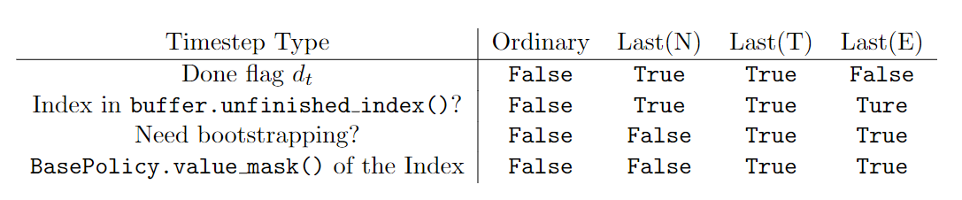
Secondly, you must know when to stop bootstrapping. Usually we stop bootstrapping when we meet a done flag. However, in the buffer above, the last (10th) step is not marked by done=True, because the collecting has not finished. We must know all those unfinished steps so that we know when to stop bootstrapping.

Luckily, this can be done under the assistance of buffer because buffers in Tianshou not only store data, but also help you manage data trajectories.

unfinished_indexes = dummy_buffer.unfinished_index()
print("unfinished_indexes: ", unfinished_indexes)
done_indexes = np.where(batch.done)[0]
print("done_indexes: ", done_indexes)
stop_bootstrap_ids = np.concatenate([unfinished_indexes, done_indexes])
print("stop_bootstrap_ids: ", stop_bootstrap_ids)

unfinished_indexes:  [9]
done_indexes:  [2]
stop_bootstrap_ids:  [9 2]

Thirdly, there are some special indexes which are marked by done flag, however its value for obs_next should not be zero. It is again because done does not differentiate between terminated and truncated. These steps are usually those at the last step of an episode, but this episode stops not because the agent can no longer get any rewards (value=0), but because the episode is too long so we have to truncate it. These kind of steps are always marked with info['TimeLimit.truncated']=True in Gym.

As a result, we need to rewrite the equation above

v_s_ *= ~batch.done

to

mask = batch.info['TimeLimit.truncated'] | (~batch.done)
v_s_ *= mask

Summary#

If you already felt bored by now, simply remember that Tianshou can help handle all these little details so that you can focus on the algorithm itself. Just call BasePolicy.compute_episodic_return().

If you still feel interested, we would recommend you check Appendix C in this paper and implementation of BasePolicy.value_mask() and BasePolicy.compute_episodic_return() for details.